Methods
The following steps are usually taken in building SDM (Plot 1): (1) locations of occurrence of a species (or other phenomenon) are recorded; (2) values of climatic predictor variables at these locations are extracted; (3) the values of predictors are used to fit a model to estimate similarity to the sites of species presence/absence; (4) The model is used to predict the variances of the species distribution across an the region of interest for a future or past climate.
i. Data Collection
Using the same sampling method as Roberts & Hamann(2015), species presence-absence records of 55743 forest inventory plot of western North America (west of 100° latitude of the USA and Canada) were collected from several public data sources. Roughly 300 pseudo-absence points(mainly caused by artificial disturbances like clear-cut) in the whole dataset were identified and corrected to ensure the absence data reliable and useful for model calibration. Since the present distribution of white spruce covers a wide range of boreal forest in Canada, to fully represent the ecological niche of the species, 2000 data points were randomly sampled over the rest North America with ArcGIS v10.1. Using the present-day distribution(E. L. little, 1971) as a reference, we classified sampled points in the distribution range as presences and others as absences.
Given by the coordinates, normal(1961-1990) climate data of sample sites was generated from software ClimateWNA v4.62(Hamann et al., 2013) with the Parameter Regression of Independent Slopes Model(PRISM) interpolation method. We chose the following 10 biological relevant climatic variables as predictors for their low correlations: degree-days below 0 (DD<0); growing degree-days(over 5 degree)(DD>5); mean coldest(MCMT) and warmest(MWMT) month temperature (°C) ; mean monthly temperature differences between July and January or continentality(°C)(TD); annual(AHM) and summer(SHM) heat-moisture index; mean annual temperature(°C)(MAT) and mean annual precipitation(mm)(MAP); April to September growing season precipitation(mm)(GSP).
Given by the coordinates, normal(1961-1990) climate data of sample sites was generated from software ClimateWNA v4.62(Hamann et al., 2013) with the Parameter Regression of Independent Slopes Model(PRISM) interpolation method. We chose the following 10 biological relevant climatic variables as predictors for their low correlations: degree-days below 0 (DD<0); growing degree-days(over 5 degree)(DD>5); mean coldest(MCMT) and warmest(MWMT) month temperature (°C) ; mean monthly temperature differences between July and January or continentality(°C)(TD); annual(AHM) and summer(SHM) heat-moisture index; mean annual temperature(°C)(MAT) and mean annual precipitation(mm)(MAP); April to September growing season precipitation(mm)(GSP).
ii. Species Distribution Modeling

Plot 1. Main steps of the project methods.
1.model fitting
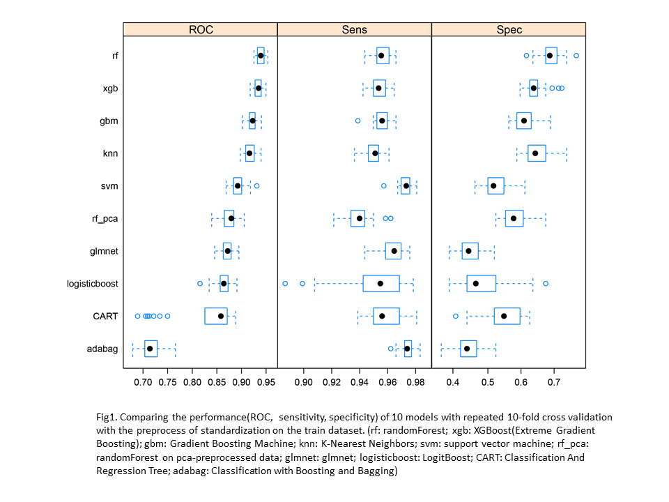
SDM is used for modeling the current distribution and then reconstructing the paleodistribution during the LGM (21000 year BP) with 2 atmosphere-ocean general circulation models(AOGCM). In this study, we fitted models with over 10 machine-learning algorithms by using CARET package(Kuhn, 2018) for R programming environment(R Core Team, 2018). Recent studies have suggested that machine-learning techniques may perform better than the traditional regression-based algorithms (Elith et al., 2006). Therefore, we used both simple regression (generalized linear model, GLM) and much more complex supervised learning approaches include Random Forest(Breiman, 2001), XGBoost(Chen & Guestrin, 2016), Gradient Boosting Machine(gbm)(Friedman, 2001), K-Nearest Neighbors(KNN)(Keller et al., 1985), support vector machine(SVM)(Suykens & Vandewalle, 1999), glmnet(Friedman et al., 2009), logistBoost(Friedman et al., 2000), Classification And Regression Trees(CART)(Breiman et al., 1984), and adaptive boosting(adabag)(Freund et al., 1999). Those algorithms are considered among the most powerful machine learning algorithms.
The SDM of current distribution was built on using 10 mentioned climatic variables of normal(1961-1990) climate as predictors and the current occurrence data of white spruce as the response variable. By standard cross-validation, the whole dataset was randomly split into two: 70% as training dataset for building models and the rest 30% as testing dataset for model evaluation. To further tune model hyperparameters and to increase the performance of the model 10-fold cross-validation was applied on the training dataset. Based on the results of the cross-validation(Fig 1), we can estimate the relative goodness of each algorithm.
The SDM of current distribution was built on using 10 mentioned climatic variables of normal(1961-1990) climate as predictors and the current occurrence data of white spruce as the response variable. By standard cross-validation, the whole dataset was randomly split into two: 70% as training dataset for building models and the rest 30% as testing dataset for model evaluation. To further tune model hyperparameters and to increase the performance of the model 10-fold cross-validation was applied on the training dataset. Based on the results of the cross-validation(Fig 1), we can estimate the relative goodness of each algorithm.
2. model validation

Fig 2. A: AUC of all models assessed by testing dataset (30% of whole data points). Five SDM algorithms selected for ensembling projections of white spruces distribution during LGM are highlighted in red color. B: ROC curve of RandomForest model with the testing dataset. Error bars represent 95% confidence intervals. AUC of the model is 87.7%, and its 95% CI range is between 87% and 88.5%. C: Importance of variables of RandomForest model based on Gini Index. Higher the values, greater the influence of variances to the model’s performance.
Next, we applied the area under the curve(AUC) of the receiver operating characteristic (ROC) to qualify the performance of fitted models by estimating the test error rate on the prior unseen dataset (testing dataset). In general, the presence thresholds of models are between 0.35 to 0.4, and the models are proved to have decent performance(AUC values are all above 0.7)(Fig 2A). Random Forest Algorithm, a learning method operating by ensemble outputs of lots of decision trees, has the highest AUC values (Fig 2B) which suggesting it has the better understanding of the ecological niche requirement of white spruce and make more reasonable predictions of the species occurrence than other models. The importance(based on Gini index) of each predictor variable can be found in Fig 2C. It indicates white spruce is sensitive to cold temperature.
3. projections
We made palaeoclimate reconstructions from 6000, 9000, 11000, 14000, 16000, and 21000 years before the present from 2 atmosphere-ocean general circulation models(AOGCM): community climate model (CCM1) and the Geophysical Fluid Dynamics Laboratory model(GFDL). Palaeoclimate data were generated by overlaying the temperature and precipitation of the palaeoclimatic model as anomalies on the high-resolution 1961-1990 climate grid.
Afterward, we predicted the probabilities of presence of white spruce for each modeling method given by palaeoclimate data under each time period available in each AOGCM. Radiocarbon-dated fossil pollen records generated from Neotoma Palaeoecology Dataset (https://www.neotomadb.org/) were used to validate the projections by the AUC values. Potential historical distribution were mapped on each palaeoecological conditions. Since a few methods do not have very good predictions on the historical distribution, we kept 5 methods (randomforest, xgbtree, svm, glm and glmnet) in the end. Despite claims of superiority of any techniques, studies have shown that projections by alternative models can be so variable(Pearson et al., 2006). To reduce the uncertainty caused by climatic models and statistical algorithms, we ensembled the projections of these 5 methods with the palaeoclimate data from 2 AOGCM.
Afterward, we predicted the probabilities of presence of white spruce for each modeling method given by palaeoclimate data under each time period available in each AOGCM. Radiocarbon-dated fossil pollen records generated from Neotoma Palaeoecology Dataset (https://www.neotomadb.org/) were used to validate the projections by the AUC values. Potential historical distribution were mapped on each palaeoecological conditions. Since a few methods do not have very good predictions on the historical distribution, we kept 5 methods (randomforest, xgbtree, svm, glm and glmnet) in the end. Despite claims of superiority of any techniques, studies have shown that projections by alternative models can be so variable(Pearson et al., 2006). To reduce the uncertainty caused by climatic models and statistical algorithms, we ensembled the projections of these 5 methods with the palaeoclimate data from 2 AOGCM.
iii. Quantitative Genetics (common garden)
Provenance trail is one standard method to understand the phenotype variances among populations, but it can also be used to estimate within-population variances by residual variances component. White spruce seed material was collected from 33 provenances along its widespread distribution and planted in Calling Lake, Alberta, CA in 5 blocks in 1978. Within each block, 5 individuals from each provenance were planted in one row. 33 provenances were grouped into 5 regions based on their climate similarity via principal component analysis with FactoMineR package(Sebastien et al., 2008) for the R v3.4.4(R Core Team, 2018).
Tree height and diameter at breast height(DBH) were measured for all 825 samples at age 12, 21, and 32. Cold hardiness of samples was also measured in 2017 by assessing the needle frozen damage level under -30 degree(Sebastian‐Azcona et al., unpublished results). Considering all seeds were planted in the same site under the identical growing condition, phenotypical differences should be driven by genetic variances. Therefore, the level of genetic diversity within population can be represented by residual variances component. We applied linear mixed models for these measurements of each region with PROC MIXED of the SAS software(SAS Institute Inc., Cary, NC, USA.). For each model, provenance and block were seen as random effects.
Tree height and diameter at breast height(DBH) were measured for all 825 samples at age 12, 21, and 32. Cold hardiness of samples was also measured in 2017 by assessing the needle frozen damage level under -30 degree(Sebastian‐Azcona et al., unpublished results). Considering all seeds were planted in the same site under the identical growing condition, phenotypical differences should be driven by genetic variances. Therefore, the level of genetic diversity within population can be represented by residual variances component. We applied linear mixed models for these measurements of each region with PROC MIXED of the SAS software(SAS Institute Inc., Cary, NC, USA.). For each model, provenance and block were seen as random effects.
