Results & Discussion
I. Verify Beringia refugium by species distribution models
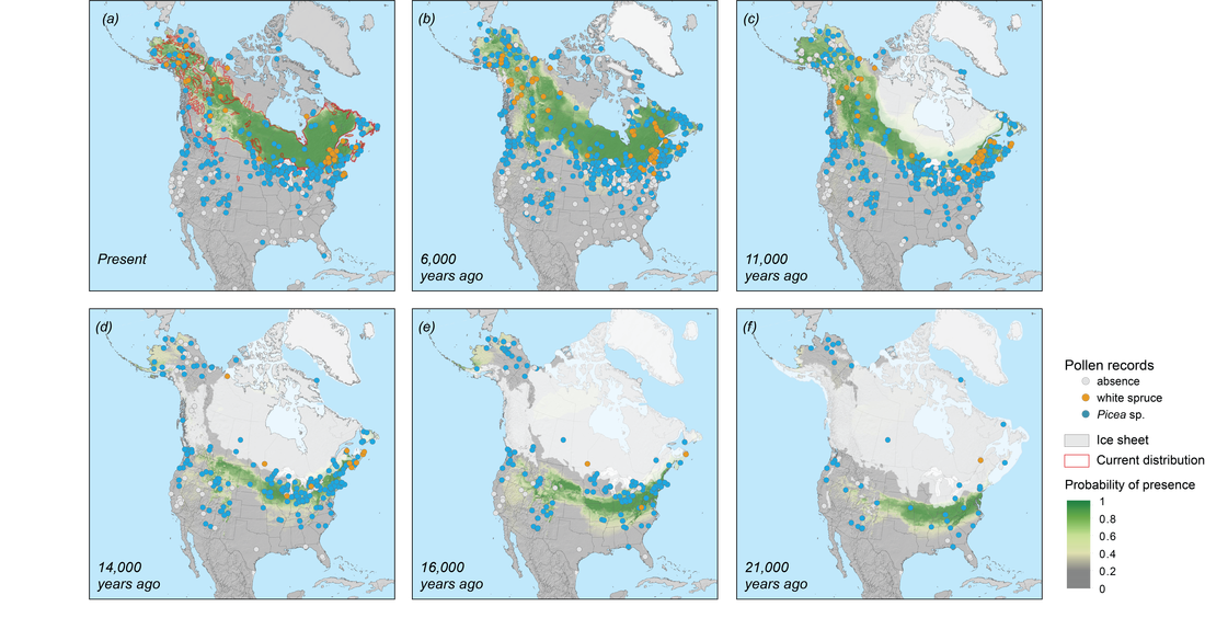
Fig 8. Maps of the projected probability of presence of white spruce for the present day (1961-1990) and the CCM1 climate reconstructions for (b) 6000,(c) 11000, (d) 14000, (e) 16000, and (f) 21000 calendar years ago with the fitted randomForest model. The current species range in (a) was from Little (1971), and the glacial ice cover shapefiles for each period were guided by Dyke et al.(2003). The historical distribution maps were made with ArcGIS v10.1(https://www.esri.com/en-us/home)
Based on the AUC values of validating testing dataset, randomForest(AUC = 0.87) seems to have the best performance on identifying the ecological niche of white spruce comparing with others(most AUC between 0.7 to 0.8). With the randomForest model, projected current distribution on 1961-1990 climate data nicely fit the present-day species range(Fig 8a). The reconstructed palaeodistribution(Fig 8) indicate the expansion of potentially suitable habitat from the eastern US to the northwestern direction as the ice sheets receded. Then the white spruce distribution reached Alaska and Yukon region, and eventually covered the current boreal forest area. During last glacial maximum(Fig 8f), potential refugia for white spruce were separated by the glacial ice and distributed at two sides of it. Besides the eastern US, small regions at the southwestern US could also had similar climate as current boreal forest region. Meanwhile, very limited extent of current Alaska may had suitable climatic condition to meet the ecological niche of white spruce, although the probability of presence is just over the threshold of the model(0.4). Therefore, according to projected distribution map at LGM, restricted zones in current Alaska may serve as refugia and harbored white spruce populations with a relatively low probability of presence. Other evidence is needed to decide the existence of Beringian refugium.
Meanwhile, the AUC yielded from against model hindcasts with palaeoecological data is lower compared with the those with the testing dataset. Still, using the randomForest model as an example, the AUC value with pollen records for the present-day and 21Ka is only 0.72 and 0.61 respectively. Firstly, although not directly used to fit models, the testing dataset is not ideally independent of the training dataset. The spatial and temporal autocorrelation among training and testing datasets partially explains the differences among AUC values. Moreover, the reliability of fossil pollen data is usually problematic. Accurately identify and date pollen are still not easy(Gavin et al., 2014). High dispersibility of pollen also increases the uncertainty of AUC values.
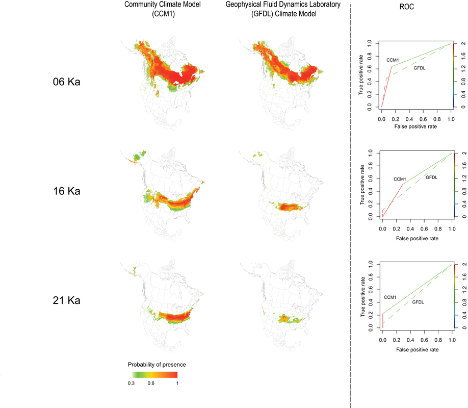
Fig 9. Projections variances of AOGCMs at each time period. With the same randomForest model, climate habitat reconstructions on 2 GCMs (CCM1 and GFDL) for 6000, 16000, and 21000 years before present. Mapped projections were evaluated by against fossil Picea pollen data of that period.
Model hindcasts are determined by changes in climate variables in a statical model. The climatic models at LGM are uncertain and generated with variances simulations. Therefore, differences between historical climatic models could cause great influences on model predictions of species palaeodistribution and habitat shift(Fig 9). Projections estimated by climate data from CCM1 seems to identify greater potential distribution range than the projections by GFDL. Also for all 3 time period, predicted habitat for CCM1 has higher AUC , which suggests the simulated climate data from CCM1 may be closer to the real historical climate condition than the ones from GFDL. To ensure the quality of projections, we need to explore alternative historical climatic models.

Fig 10. AUC values of projections for each modeling method given by palaeoclimate data under each time period available in each AOGCM. We use historical climatic condition from CCM1 for 6000, 11000, 14000, 16000, and 21000 years BP and from GFDL for 6000, 9000, 14000, 16000, and 21000 years BP.
Besides RandomForest, the rest models have similar projection variances among AOGCMs of each time period. With the same modeling technique, the projections for CCM1 tend to fit pollen data better than the ones for GFDL climatic model exception of around 11000 years BP period(Fig 10). This AUC variances pattern among AOGCMs indicates that in general CCM1 fits the real historical climate better than GFDL.
In addition to AOGCMs, modeling methods can contribute the uncertainty of projections. We usually use present-day data to evaluate one model, but the performance of each modeling may change through time(Fig 10). The patterns of AUC for randomForest(RF), xgbtree, and SVM under CCM1(solid lines in Fig 10) are similar: AUC decreases with the time period away from the present. All the three techniques reached relatively high AUC(over 0.7) for the present projections; then, the AUC drops to 0.6 or even lower for the LGM period. Meanwhile, GLM and Glment under CCM1 have the opposite trend: relatively low AUC for the present projections and have even higher AUC values as time increases. Hence, assessing methods based on present data may not always reflect the performance of a given (temporal/spacial) situation.

Fig 11. The probability of presence during LGM estimated from 10 projections.
Araujo and New(2006) advice ensemble predictions is helpful to achieve more robust predictions. To reduce the uncertainties introduced by AGOCMs and modeling techniques, we committed a simple unweighted average of the predictions for ensemble the probability of presence from all projections. The ensemble habitat distribution from 10 projections(5 modeling techniques * 2 AOGCMs) should reduce the ‘noise’ associated with individual model uncertainties(Forester et al., 2013).
According to Fig 11, western and eastern Alaska regions have at least 30% probability of presence. Thus, our climate habitat reconstruction supports eastern Beringia(current Alaska) could have generally suitable climate condition to be used as refugia for white spruce during LGM. Low-frequency Picea pollen is present in Eastern Beringia region around 21000 years BP(Fig 11a). Brukaker et al.(2005) found Picea pollen is absent in western Beringia area at that period, so it is unlikely that Picea pollen is from the Siberia region through long-distance dispersal. Macrofossils of Picea spp. were also available in Eastern Beringia at that time (Zazula et al., 2006). The most pollen records clustered in the north-central area of Alaska, where have some small regions with potentially suitable climate for white spruce population based on our climate habitat reconstruction. By the utility of nuclear microsatellites and chloroplast DNA, Anderson et al.(2006, 2013) believe north-central Alaska served as a glacial refugium at LGM. Taken together, these evidences support our hypothesis that there was Beringian refugium for white spruce during the last glacial maximum period, although the glacial refuge population in Alaska is supposed to be small and isolated as its low number of palaeoecological data suggest.
II. Quantitative genetics

Fig 12. Locations of 33 populations and the test site of the provenance trail.

Table 1. residual variances component of growth and adaptive traits by region. Standard errors of residual variances component are shown in parentheses.
Residual variances components of growing traits by regions prove the white spruce samples from central, eastern coastal, and southern Ontario have the highest genetic diversity in the majority of measured quantitative traits(Table 1). In all the measured traits, Yukon is the least genetically diverse region; the residual variances components of Yukon is much lower than other regions. All region besides Yukon are fairly homogeneous in tree height at age 12, and the variances of tree heights become more obvious at age 32. In general, the level of genetic diversity decrease from the eastern coast to Yukon area.
If eastern Beringia severed as refugia for white spruce at LGM, refuge populations should have high genetic diversity and unique alleles; On the contrary, Yukon region is geographically close to eastern Beringia but have incredibly low genetic diversity in all measured traits. Phylogeography analysis with nuclear microsatellites(Anderson et al., 2013) and chloroplast DNA(Anderson et al., 2006) reveal that current white spruce populations in Alaska do have high genetic diversity and unique alleles and haplotypes versus outside Alaska populations. One possible explanation is northwestern cordillera mountains as a geographic barrier(Stralbert et al., 2017) limit the gene flow among Alaska and non-Alaska populations. Therefore, although neighboring to Alaska, Yukon population may have been derived from the southern refugia and have different genetic lineages to the Alaska refuge populations. After repeated founder effects, the genetic diversity of Yukon populations shrank dramatically during the post‐glacial migration.
Residual variances of components of central and eastern Canada are both high. The genetic discontinuity is very common in widespread North American boreal species, black spruce (Jaramillo‐Correa et al., 2004) and jack pine(Godbout et al., 2005). The observed genetic discontinuity can be explained by the division of different eastern lineages; one mitigated to eastern Quebec and Maritime Provinces of Canada, and the other lineage distributed from the Great Lakes to the Rocky Mountains. By Lafontaine et al.(2010), white spruce populations can be classified into three groups(west, central and east) by allelic richness, which means there are three lineages for these three groups. Western group is the Alaska group, long-term isolation in Beringia refugium can explain the unique alleles in western group. According to the climate habitat reconstructions for 21000 years BP, a wide range of refugium of white spruce at the eastern US. Studies prove the discontinuity between the populations on both sides of the Appalachian Mountains(Mylecraine et al., 2004). Two slopes of the Mountains could be the source of two lineages.

Fig 12. General pattern of post glacial migration.
